Reading Microclimatic Data
myClim natively supports the import of several pre-defined loggers.
You can view the list of pre-defined loggers using
names(myClim::mc_data_formats). To specify the data format
when reading files, set the dataformat_name parameter.
There is also the possibility to read user-defined loggers by defining
the user_data_formats parameter. For examples of how to
read custom loggers in myClim, please refer to a separate vignette.
Alternatively, myClim can read records from any wide or long data frame
in R.
The mc_read_files(), mc_read_wide(), and mc_read_long() functions can be used for reading in data without metadata. These functions are user-friendly, fast, and allow for exploratory data analysis. myClim automatically organizes data into artificial localities, and metadata can be updated at a later stage. To organize records into real localities and provide metadata, use the mc_read_data() function along with two tables:1. A table that specifies logger file paths, data format name, logger type, and locality. 2. A table that provides locality metadata, such as coordinates, elevation, time offset to UTC, and so on.
library(myClim)
## Read pre-defined loggers without metadata
# read from Tomst files
tms.f <- mc_read_files(c("data_91184101_0.csv", "data_94184102_0.csv",
                         "data_94184103_0.csv"),
                       dataformat_name = "TOMST", silent = T)

# read from HOBO files
hob.f <- mc_read_files(c("20024354_comma.csv"),
                       dataformat_name = "HOBO",
                       date_format = "%y.%m.%d %H:%M:%S",
                       silent = T)

# read all Tomst files from current directory
tms.d <- mc_read_files(".", dataformat_name = "TOMST", recursive = F, silent = T)

# read from data.frame
meteo.table <- readRDS("airTmax_meteo.rds") # wide format data frame
meteo <- mc_read_wide(meteo.table, sensor_id = "T_C",
                      sensor_name = "airTmax", silent = T)

## Read pre-defined logger with metadata
# provide two tables. Can be csv files or R data.frame
ft <- read.table("files_table.csv", sep=",", header = T)
lt <- read.table("localities_table.csv", sep=",", header = T)

tms.m <- mc_read_data(files_table = "files_table.csv",
                      localities_table = lt,
                      silent = T)
Pre-Processing
-
Cleaning Time Series:
mc_prep_clean()corrects time-series data if it is in the wrong order, contains duplicates, or has missing values. The cleaning log is saved in the myClim object and can be accessed usingmc_info_clean()after cleaning. By default, cleaning is performed during reading.
# clean runs automatically while reading
tms <- mc_prep_clean(tms.m, silent = T) # clean series
#> Warning in mc_prep_clean(tms.m, silent = T): MyClim object is already cleaned.
#> Repeated cleaning overwrite cleaning informations.
tms.info <- mc_info_clean(tms) # call cleaning log-
Handling time zones: myClim expects input data to
be in UTC time. However, it is ecologically meaningful to use solar time
instead, as it respects local photoperiods, especially when working with
global datasets. The
mc_prep_solar_tz()function calculates solar time from the longitude of the locality. Besides solar_tz the offset can be also set manually usingmc_prep_meta_locality()to respect e.g. political time.
tms <- mc_prep_solar_tz(tms) # calculate solar time

# provide user defined offset to UTC in minutes
# for conversion to political time use offset in minutes.
tms.usertz <- mc_prep_meta_locality(tms,
                                    values = as.list(c(A1E05 = 60,
                                                       A2E32 = 0,
                                                       A6W79 = 120)),
param_name = "tz_offset")-
Sensor calibration: If your sensor is recording
values that are warmer or colder than the true values, and you know the
amount of the discrepancy, you can correct the measurements by adding
the offsets (+/-). Use
mc_prep_calib_load()to upload the offsets into the myClim object, and then usemc_prep_calib()to apply the offset correction.
# simulate calibration data (sensor shift/offset to add)
i <- mc_info(tms)
calib_table <- data.frame(serial_number = i$serial_number,
                          sensor_id     = i$sensor_id,
                          datetime      = as.POSIXct("2016-11-29",tz="UTC"),
                          cor_factor    = 0.398,
                          cor_slope     = 0)

## load calibration to myClim metadata
tms.load <- mc_prep_calib_load(tms, calib_table)

## run calibration for selected sensors
tms <- mc_prep_calib(tms.load, sensors = c("TM_T",
                                           "TMS_T1",
                                           "TMS_T2",
"TMS_T3"))-
Info functions: For data overview use:
-
mc_info_count()which returns the number of localities, loggers and sensors in myClim object -
mc_info()returning data frame with summary per sensor -
mc_info_meta()returning the data frame with locality metadata -
mc_info_clean()returning the data frame with cleaning log
-
mc_info_count(tms)
mc_info_clean(tms)
mc_info(tms)
Example output table of mc_info()
| locality_id | serial_number | sensor_id | sensor_name | start_date | end_date | step_seconds | period | min_value | max_value | count_values | count_na | height | calibrated |
|---|---|---|---|---|---|---|---|---|---|---|---|---|---|
| A1E05 | 91184101 | Thermo_T | Thermo_T | 2020-10-28 08:45:00 | 2021-04-18 07:30:00 | 900 | NA | -15.94 | 22.69 | 16508 | 0 | air 200 cm | FALSE |
| A2E32 | 94184103 | TMS_T1 | TMS_T1 | 2020-10-16 06:15:00 | 2021-04-13 09:15:00 | 900 | NA | 2.52 | 11.40 | 17197 | 0 | soil 8 cm | TRUE |
| A2E32 | 94184103 | TMS_T2 | TMS_T2 | 2020-10-16 06:15:00 | 2021-04-13 09:15:00 | 900 | NA | -0.60 | 13.77 | 17197 | 0 | air 2 cm | TRUE |
| A2E32 | 94184103 | TMS_T3 | TMS_T3 | 2020-10-16 06:15:00 | 2021-04-13 09:15:00 | 900 | NA | -8.98 | 24.52 | 17197 | 0 | air 15 cm | TRUE |
| A2E32 | 94184103 | TMS_moist | TMS_moist | 2020-10-16 06:15:00 | 2021-04-13 09:15:00 | 900 | NA | 1996.00 | 2780.00 | 17197 | 0 | soil 0-15 cm | FALSE |
| A6W79 | 94184102 | TMS_T1 | TMS_T1 | 2020-10-06 09:00:00 | 2021-04-07 11:45:00 | 900 | NA | 1.27 | 12.65 | 17580 | 0 | soil 8 cm | TRUE |
| A6W79 | 94184102 | TMS_T2 | TMS_T2 | 2020-10-06 09:00:00 | 2021-04-07 11:45:00 | 900 | NA | -4.85 | 14.40 | 17580 | 0 | air 2 cm | TRUE |
| A6W79 | 94184102 | TMS_T3 | TMS_T3 | 2020-10-06 09:00:00 | 2021-04-07 11:45:00 | 900 | NA | -14.41 | 19.65 | 17580 | 0 | air 15 cm | TRUE |
| A6W79 | 94184102 | TMS_moist | TMS_moist | 2020-10-06 09:00:00 | 2021-04-07 11:45:00 | 900 | NA | 1257.00 | 2939.00 | 17580 | 0 | soil 0-15 cm | FALSE |
- Cropping, filtering, and merging:
## crop the time-series
start <- as.POSIXct("2021-01-01", tz = "UTC")
end   <- as.POSIXct("2021-03-31", tz = "UTC")

tms   <- mc_prep_crop(tms, start, end)


## simulate another myClim object and rename some localities and sensors
tms1 <- tms
tms1 <- mc_prep_meta_locality(tms1, list(A1E05 = "ABC05", A2E32 = "CDE32"),
                              param_name = "locality_id") # locality ID

tms1 <- mc_prep_meta_sensor(tms1,
                            values=list(TMS_T1 = "TMS_Tsoil",
                                        TMS_T2 = "TMS_Tair2cm"),
                            localities = "A6W79", param_name = "name") # sensor names

## merge two myClim objects Prep-format
tms.m  <- mc_prep_merge(list(tms, tms1))
tms.im <- mc_info(tms.m) # see info

## Filtering
tms.out  <- mc_filter(tms, localities = "A1E05", reverse = T) # exclude one locality.
tms.m    <- mc_filter(tms.m, sensors = c("TMS_T2", "TMS_T3"), reverse = F) # keep only two sensor
tms.if <- mc_info(tms.m) # see info -
Updating metadata: To update locality metadata, use
mc_prep_meta_locality(). With this function, users can rename the locality, set the time offset, adjust the coordinates, elevation, and other metadata. For updating sensor metadata, usemc_prep_meta_sensor(), which allows users to rename the sensor and update the sensor’s height or depth. Many sensors have a predefined height, which is important for data joining.
## upload metadata from data frame

# load data frame with metadata (coordinates)
metadata <- readRDS("metadata.rds")

# upload metadata from data.frame
tms.f <- mc_prep_meta_locality(tms.f, values = metadata)

## upload metadata from named list
tms.usertz <- mc_prep_meta_locality(tms,
                                    values = as.list(c(A1E05 = 57,
                                                            A2E32 = 62,
                                                            A6W79 = 55)),
                                    param_name = "tz_offset")
Metadata table ready for mc_prep_meta_locality()
| locality_id | lat_wgs84 | lon_wgs84 |
|---|---|---|
| 91184101 | 50.90 | 14.24 |
| 94184103 | 50.95 | 14.09 |
| 94184102 | 50.93 | 14.32 |
-
Joining in time To join fragmented time-series that
are stored in separate files from separate downloading visits of the
localities, use
mc_join().
# one locality with two downloads in time
data <- mc_load("join_example.rds")

joined_data <- mc_join(data, comp_sensors = c("TMS_T1", "TMS_T2"))

#> Locality: 94184102
#> Problematic interval: 2020-12-01 00:00:00 UTC--2020-12-31 23:45:00 UTC
#>
#> Older logger TMS 94184102
#> start                 end
#> 2020-10-06 09:15:00   2020-12-31 23:45:00
#>
#> Newer logger TMS 94184102
#> start                end
#> 2020-12-01 00:00:00  2021-04-07 11:45:00
#>
#> Loggers are different. They cannot be joined automatically.
#>
#> 1: use older logger
#> 2: use newer logger
#> 3: use always older logger
#> 4: use always newer logger
#> 5: exit
#>
#> Write choice number or start datetime of use newer
#> logger in format YYYY-MM-DD hh:mm.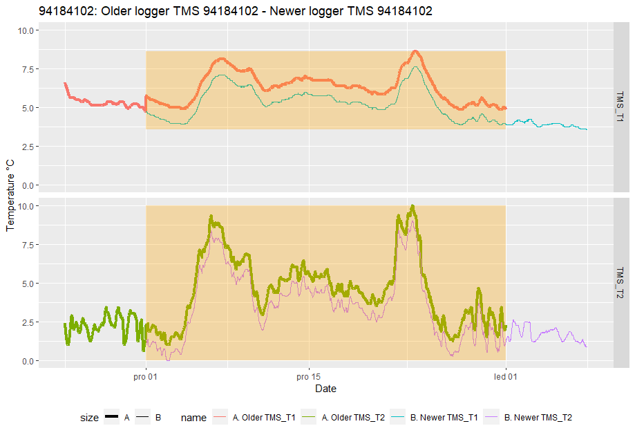
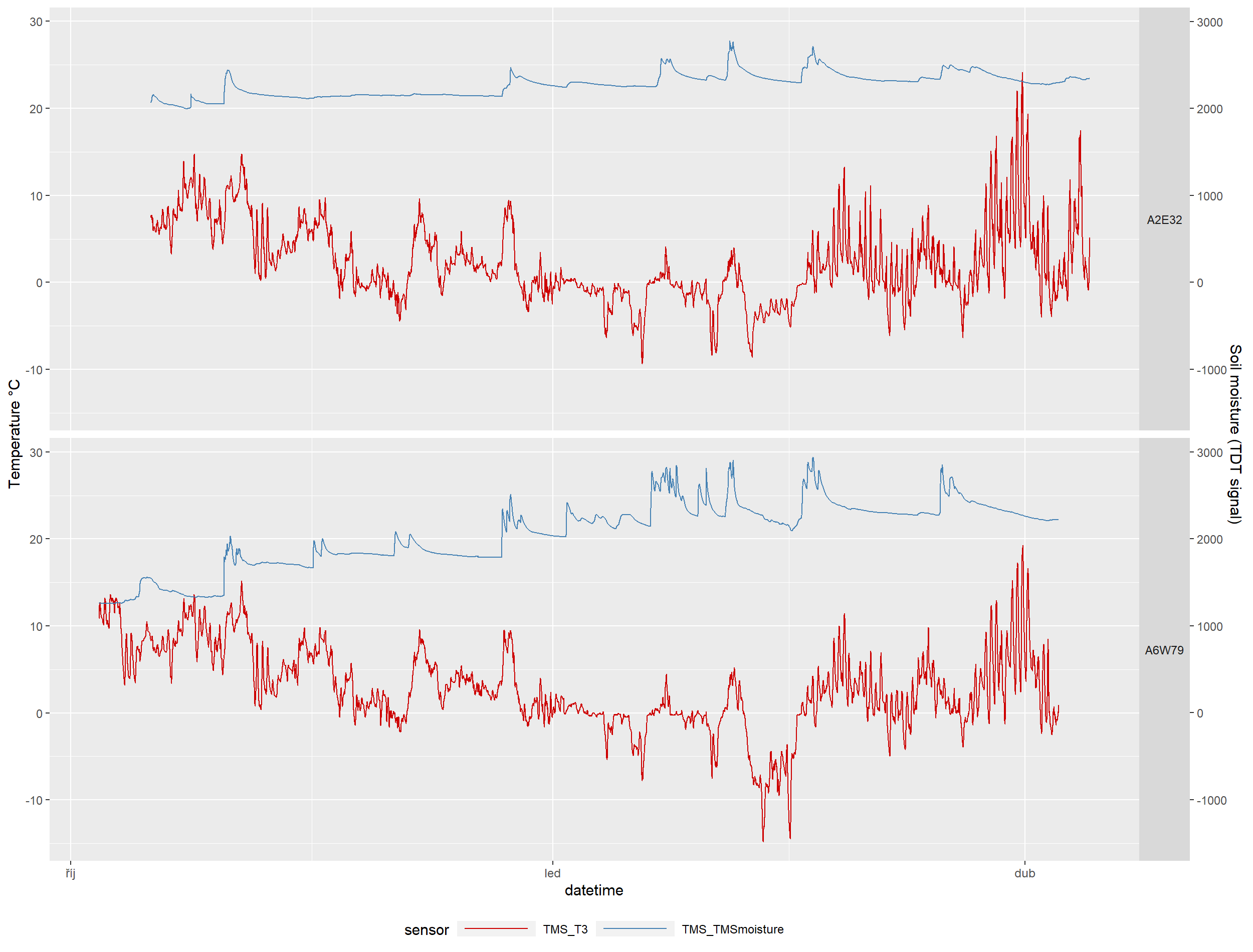
Plotting
You can create a raster plot using mc_plot_raster() or a
line time series plot using mc_plot_line(). The line time
series plot supports a maximum of two different physical units (e.g.,
temperature and soil moisture) that can be plotted together on the
primary and secondary y-axes. The plotting functions return a ggplot
object that can be further adjusted with ggplot syntax or can be saved
directly as PDF or PNG files on your drive.
## lines
tms.plot <- mc_filter(tms, localities = "A6W79")

p <- mc_plot_line(tms.plot, sensors = c("TMS_T3", "TMS_T1", "TMS_moist"))
p <- p+ggplot2::scale_x_datetime(date_breaks = "1 week", date_labels = "%W")
p <- p+ggplot2::xlab("week")
p <- p+ggplot2::aes(size = sensor_name)
p <- p+ggplot2::scale_size_manual(values = c(1, 1 ,2))
p <- p+ggplot2::guides(size = "none")
p <- p+ggplot2::scale_color_manual(values = c("hotpink", "pink", "darkblue"), name = NULL)

## raster
mc_plot_raster(tms, sensors = c("TMS_T3"))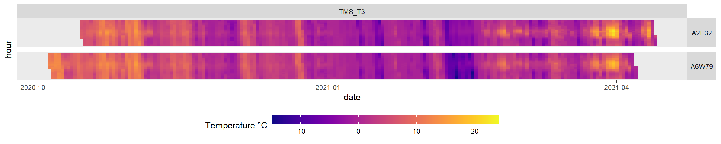
Aggregation
Using the mc_agg() function, you can aggregate
time-series data (e.g., from 15-minute intervals) into hourly, daily,
weekly, monthly, seasonal, or yearly intervals using various functions
such as mean, max, percentile, sum, and more.
# with defaults only convert Raw-format  to Agg-format
tms.ag <- mc_agg(tms.m,fun = NULL, period = NULL)

# aggregate to daily mean, range, coverage, and 95 percentile.
tms.day <- mc_agg(tms, fun = c("mean", "range", "coverage", "percentile"),
                percentiles = 95, period = "day", min_coverage = 0.95)

# aggregate all time-series, return one value per sensor.
tms.all <- mc_agg(tms, fun = c("mean", "range", "coverage", "percentile"),
                percentiles = 95, period = "all", min_coverage = 0.95)

# aggregate with your custom function. (how many records are below -5°C per month)
tms.all.custom <- mc_agg(tms.out, fun = list(TMS_T3 = "below5"), period = "month",
                         custom_functions = list(below5 = function(x){length(x[x<(-5)])}))
r <- mc_reshape_long(tms.all.custom)
Calculation
Within myClim object it is possible to calculate new virtual sensors (i.e., microclimatic variables), such as volumetric water content, growing and freezing degree days, and snow cover duration, among others.
## calculate virtual sensor VWC from raw TMS moisture signal
tms.calc <- mc_calc_vwc(tms.out, soiltype = "loamy sand A")

## virtual sensor with growing and freezing degree days
tms.calc <- mc_calc_gdd(tms.calc, sensor = "TMS_T3",)
tms.calc <- mc_calc_fdd(tms.calc, sensor = "TMS_T3")

## virtual sensor to estimate snow presence from 2 cm air temperature
tms.calc <- mc_calc_snow(tms.calc, sensor = "TMS_T2")

## summary data.frame of snow estimation
tms.snow <- mc_calc_snow_agg(tms.calc)

##  virtual sensor with VPD
hobo.vpd <- mc_calc_vpd(hob.f)
Output table of mc_calc_snow_agg
| locality_id | snow_days | first_day | last_day | first_day_period | last_day_period |
|---|---|---|---|---|---|
| A2E32 | 13 | 2021-02-06 | 2021-02-18 | 2021-02-06 | 2021-02-18 |
| A6W79 | 14 | 2021-01-11 | 2021-01-31 | 2021-01-11 | 2021-01-31 |
Standard myClim environmental variables
Unlike other functions that return myClim objects,
mc_env functions returns an analysis-ready flat table that
represents a predefined set of standard microclimatic variables.
mc_env_temp() for example: the 5th percentile of daily
minimum temperatures, the mean of daily mean temperatures, the 95th
percentile of daily maximum temperatures, the mean of daily temperature
range, the sum of degree days above a base temperature (default 5°C),
the sum of degree days below a base temperature (default 0°C), and the
number of days with frost (daily minimum < 0°C).
temp_env  <- mc_env_temp(tms, period = "all", min_coverage = 0.9)
moist_env <- mc_env_moist(tms.calc, period = "all", min_coverage = 0.9)
vpd_env   <- mc_env_vpd(hobo.vpd, period = "all", min_coverage = 0.9)
Reshaping
Microclimatic records from myClim objects can be converted to a wide
or long data frame using mc_reshape_wide() and
mc_reshape_long() functions. This can be useful for data
exploration, visualization, and further analysis outside of the myClim
framework. The wide format represents each sensor as a separate column
with time as rows, while the long format stacks the sensor columns and
adds additional columns for variable names and sensor IDs.
## wide table of air temperature and soil moisture
tms.wide <- mc_reshape_wide(tms.calc, sensors = c("TMS_T3", "vwc"))

## long table of air temperature and soil moisture
tms.long <- mc_reshape_long(tms.calc, sensors = c("TMS_T3", "vwc"))

tms.long.all <- mc_reshape_long(tms.all)| datetime | A2E32_1_94184103_TMS_T3 | A6W79_1_94184102_TMS_T3 |
|---|---|---|
| 2021-01-01 00:00:00 | -0.23 | 0.77 |
| 2021-01-01 00:15:00 | -0.23 | 0.77 |
| 2021-01-01 00:30:00 | -0.10 | 0.77 |
| 2021-01-01 00:45:00 | 0.02 | 0.77 |
| 2021-01-01 01:00:00 | -0.10 | 0.84 |
| 2021-01-01 01:15:00 | -0.29 | 0.90 |
| 2021-01-01 01:30:00 | -0.35 | 1.02 |
| 2021-01-01 01:45:00 | -0.23 | 1.02 |
| 2021-01-01 02:00:00 | -0.23 | 1.09 |
| 2021-01-01 02:15:00 | -0.16 | 1.09 |
| locality_id | serial_number | sensor_name | height | datetime | time_to | value |
|---|---|---|---|---|---|---|
| A2E32 | 94184103 | TMS_T3 | air 15 cm | 2021-01-01 00:00:00 | 2021-01-01 00:15:00 | -0.23 |
| A2E32 | 94184103 | TMS_T3 | air 15 cm | 2021-01-01 00:15:00 | 2021-01-01 00:30:00 | -0.23 |
| A2E32 | 94184103 | TMS_T3 | air 15 cm | 2021-01-01 00:30:00 | 2021-01-01 00:45:00 | -0.10 |
| A2E32 | 94184103 | TMS_T3 | air 15 cm | 2021-01-01 00:45:00 | 2021-01-01 01:00:00 | 0.02 |
| A2E32 | 94184103 | TMS_T3 | air 15 cm | 2021-01-01 01:00:00 | 2021-01-01 01:15:00 | -0.10 |
| A2E32 | 94184103 | TMS_T3 | air 15 cm | 2021-01-01 01:15:00 | 2021-01-01 01:30:00 | -0.29 |
| A2E32 | 94184103 | TMS_T3 | air 15 cm | 2021-01-01 01:30:00 | 2021-01-01 01:45:00 | -0.35 |
| A2E32 | 94184103 | TMS_T3 | air 15 cm | 2021-01-01 01:45:00 | 2021-01-01 02:00:00 | -0.23 |
| A2E32 | 94184103 | TMS_T3 | air 15 cm | 2021-01-01 02:00:00 | 2021-01-01 02:15:00 | -0.23 |
| A2E32 | 94184103 | TMS_T3 | air 15 cm | 2021-01-01 02:15:00 | 2021-01-01 02:30:00 | -0.16 |