myClim: reading user-defined loggers

In case you are NOT using one of the predefined microclimatic loggers listed in r names(myClim::mc_data_formats), you can create a user-defined myClim class using mc_data_formats. By doing this, you teach myClim how to parse your files into a myClim object.

Example files are available on GitHub.

============================================================

HOBO MX2301A bluetooth-enabled series
collected using the HOBOconnect software

# Load the 'myClim' library
library(myClim)
# Create a list to define a custom data format for 'myHOBO'
user_data_formats <- list(myHOBO=new("mc_DataFormat"))

# Set various properties for the 'myHOBO' data format
user_data_formats$myHOBO@skip <- 1 # Skip the first row
user_data_formats$myHOBO@separator <- "," # Define the separator as a comma
user_data_formats$myHOBO@date_column <- 2 # Specify the column containing dates
user_data_formats$myHOBO@date_format <- "%m/%d/%Y %H:%M:%S" # Define the date format
user_data_formats$myHOBO@tz_offset <- 2 * 60 # Set the time zone offset in minutes
user_data_formats$myHOBO@columns[[mc_const_SENSOR_T_C]] <- 3 # Map temperature to column 3
user_data_formats$myHOBO@columns[[mc_const_SENSOR_RH]] <- 4 # Map humidity to column 4

# Read data from a CSV file using the 'myHOBO' format, without cleaning
my_data <- mc_read_files("./21498648.csv", "myHOBO", clean=FALSE,
                             user_data_formats=user_data_formats)
# Clean data in myClim object
my_data_clean<-mc_prep_clean(my_data)
#> 1 loggers
#> datetime range: 2022-10-21 11:30:00 - 2022-10-22 13:00:00
#> detected steps: (1800s = 30min)
#>          locality_id serial_number          start_date            end_date
#> 21498648    21498648      21498648 2022-10-21 11:30:00 2022-10-22 13:00:00
#>          step_seconds count_duplicities count_missing count_disordered rounded
#> 21498648         1800                 5             0                0    TRUE
# Plot the cleaned data with a scale coefficient of 0.1
mc_plot_line(my_data_clean,scale_coeff = 0.1)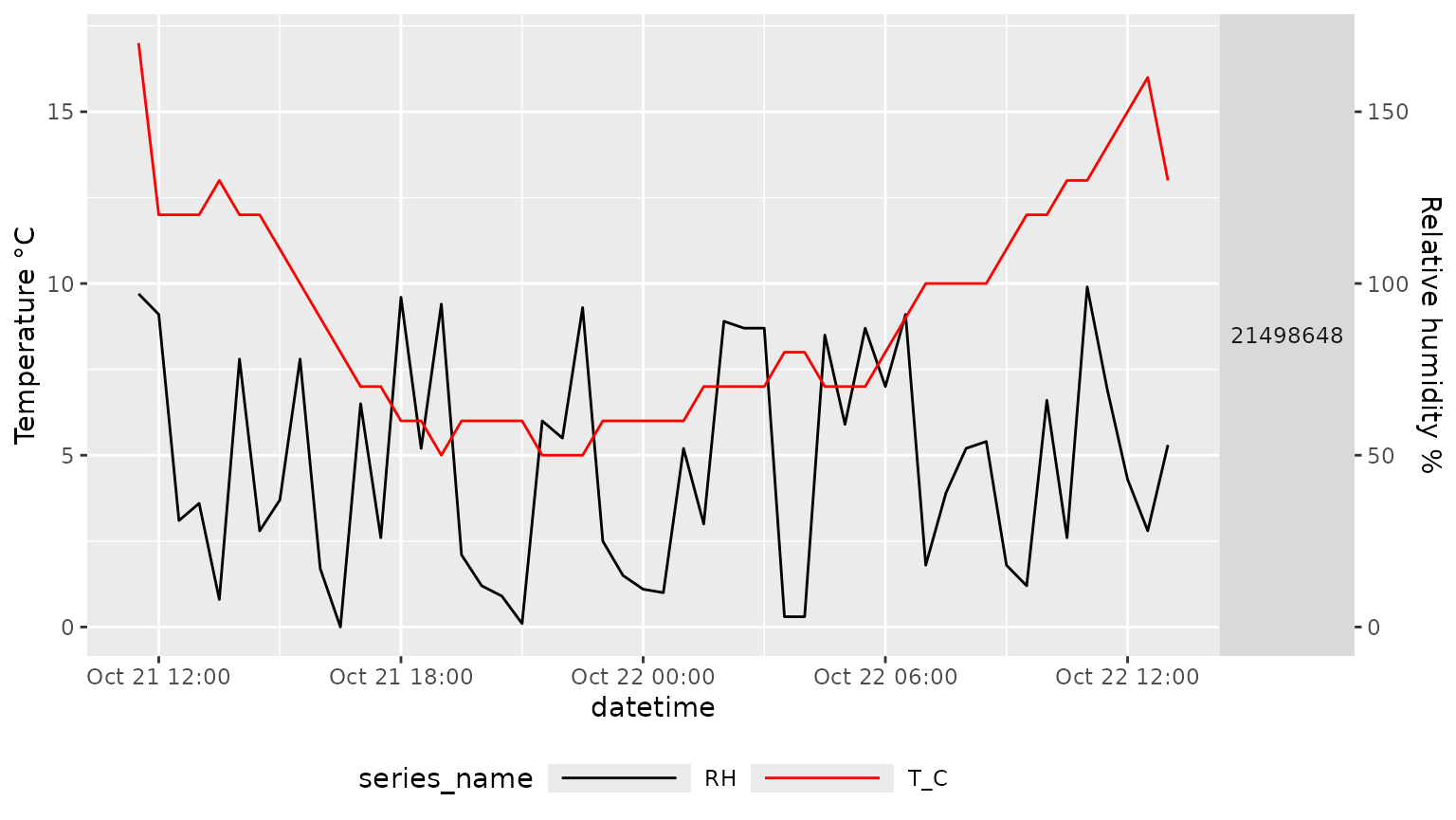  

============================================================

ElectricBlue EnvLogger TH2.5
collected using the EnvLogger Viewer App

# Load the 'myClim' library
library(myClim)
# Create a list to define a custom data format for 'my_EnvLogger'
user_data_formats <- list(my_EnvLogger=new("mc_DataFormat")) 

# Set properties for the data format
user_data_formats$my_EnvLogger@skip <- 23 # Skip the first 23 rows
user_data_formats$my_EnvLogger@separator <- "," # Define the separator as a comma
user_data_formats$my_EnvLogger@date_column <- 1 # Specify the column containing dates
user_data_formats$my_EnvLogger@date_format <- "%Y-%m-%d %H:%M:%S" # Define the date format
user_data_formats$my_EnvLogger@tz_offset <- 0 # Set the time zone offset to 0 (UTC)
user_data_formats$my_EnvLogger@columns[[mc_const_SENSOR_T_C]] <- 2 # Map temperature to column 2
user_data_formats$my_EnvLogger@columns[[mc_const_SENSOR_RH]] <- 3 # Map humidity to column 3

# Read data from a CSV file using the 'my_EnvLogger' format, without cleaning
my_data <- mc_read_files("./envloggerexample.csv", "my_EnvLogger", clean=FALSE,
                             user_data_formats=user_data_formats)
# Clean data in myClim object
my_data_clean<-mc_prep_clean(my_data)
#> 1 loggers
#> datetime range: 2023-06-24 14:30:00 - 2023-09-03 11:00:00
#> detected steps: (1800s = 30min)
#>                       locality_id    serial_number          start_date
#> envloggerexample envloggerexample envloggerexample 2023-06-24 14:30:00
#>                             end_date step_seconds count_duplicities
#> envloggerexample 2023-09-03 11:00:00         1800                 0
#>                  count_missing count_disordered rounded
#> envloggerexample             0                0   FALSE
# Plot the cleaned data with a scale coefficient of 0.1
mc_plot_line(my_data_clean,scale_coeff = 0.4)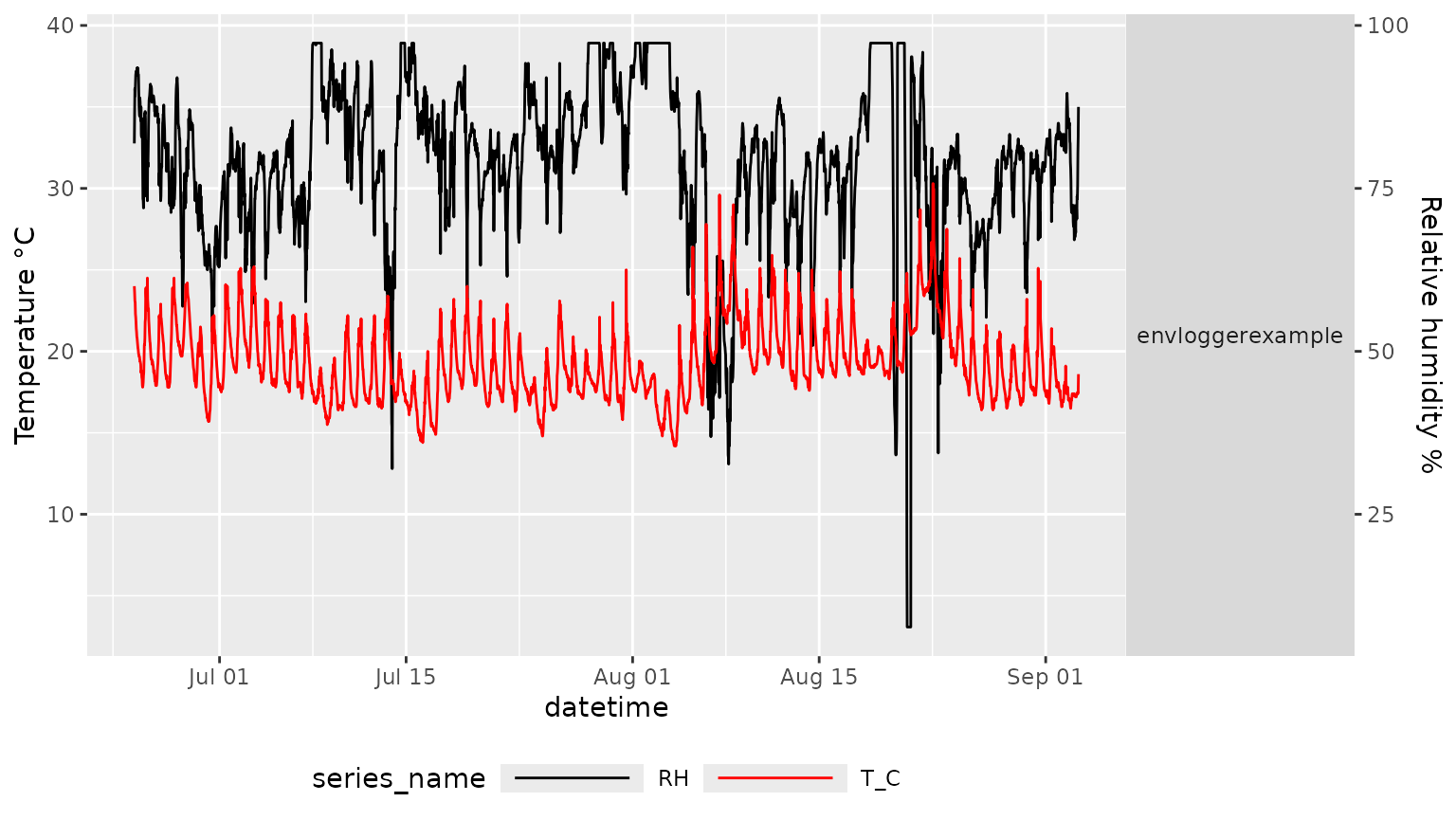  

===============================================================

artificial example
logger with soil moisture sensor and 3 temperature sensors

# Define a vector of file names
files <- c("TMS94184102.csv", "TMS94184102_CET.csv")

# Create a list to define a custom data format for 'my_logger'
user_data_formats <- list(my_logger=new("mc_DataFormat"))
user_data_formats$my_logger@date_column <- 2 # Specify the column containing dates
user_data_formats$my_logger@tz_offset <- 0 # Set the time zone offset to 0 (UTC)
user_data_formats$my_logger@columns[[mc_const_SENSOR_T_C]] <- c(3, 4, 5) # Map multiple temperature columns
user_data_formats$my_logger@columns[[mc_const_SENSOR_real]] <- 6 # Map real sensor data to column 6

# Read data from the specified files using the 'my_logger' format, with data cleaning, silently (no console output)
my_data <- mc_read_files(files, "my_logger", silent=TRUE, user_data_formats=user_data_formats)
# Plot the data with a scale coefficient of 0.01
mc_plot_line(my_data,scale_coeff = 0.01)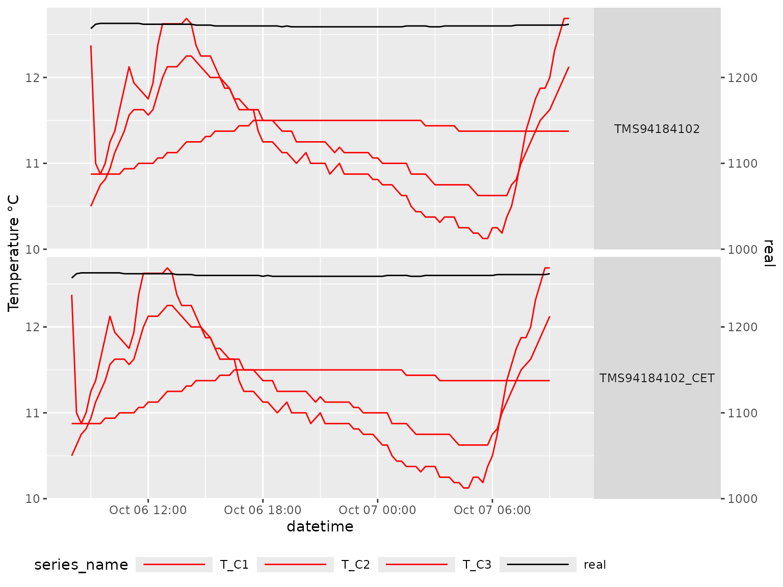 

===============================================================

Rename sensors if necessary

# Existing names
levels(factor(mc_info(my_data)[["sensor_name"]])) 
#> [1] "T_C1" "T_C2" "T_C3" "real"

# Define the new names
my_data <- mc_prep_meta_sensor(my_data,
                               list(real = "soil moisture", 
                                    T_C1 = "soil T",
                                    T_C2 = "ground T",
                                    T_C3 = "air T"),
                               param_name="name")
# Check the new names
levels(factor(mc_info(my_data)[["sensor_name"]]))
#> [1] "air T"         "ground T"      "soil T"        "soil moisture"

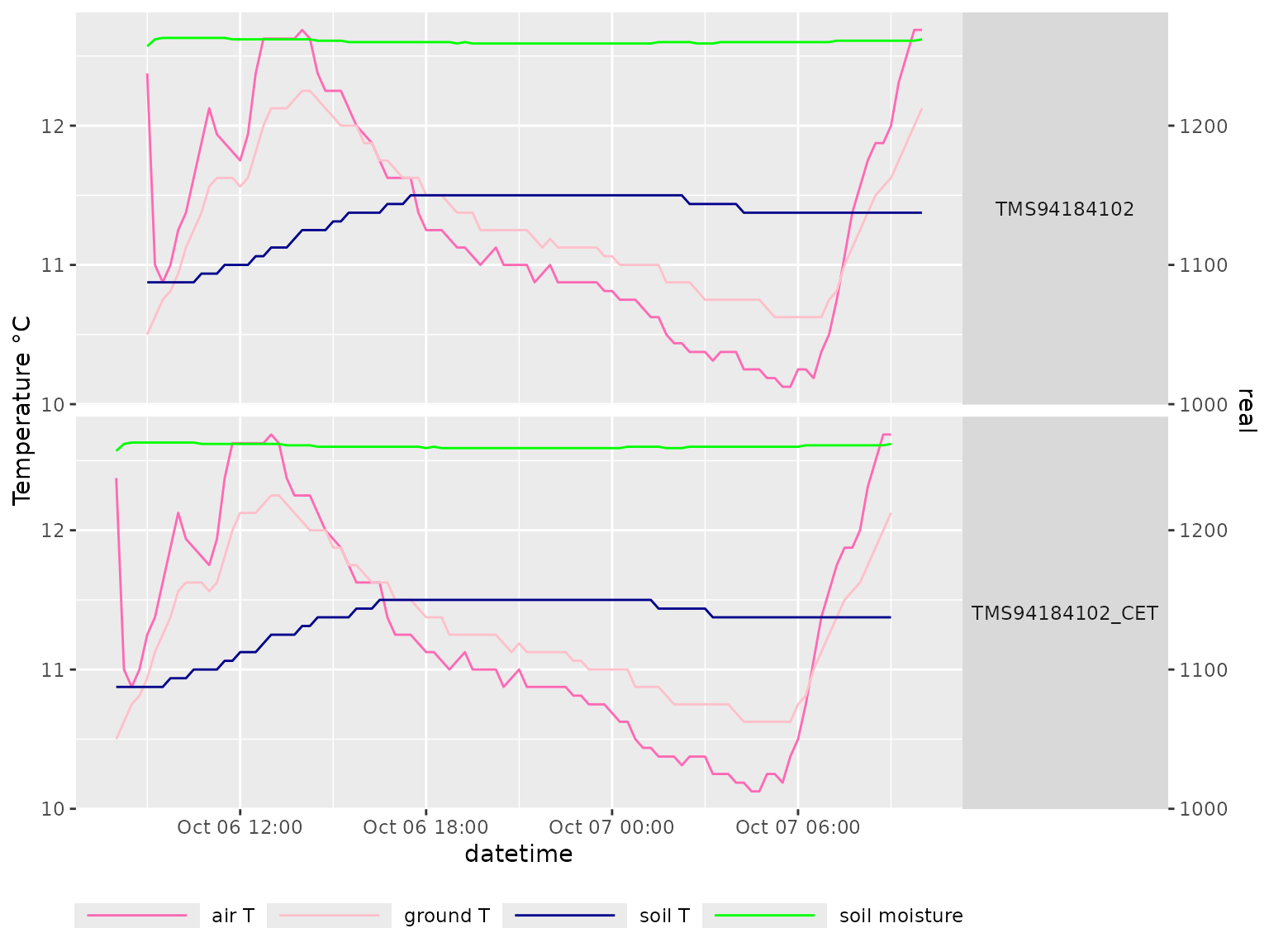
# Plot the data with a scale coefficient of 0.01
p <- mc_plot_line(my_data,scale_coeff = 0.01) 
# Modify default colors. 
p <- p+ggplot2::scale_color_manual(values=c("hotpink",
                                            "pink", 
                                            "darkblue",
                                            "green"),
                                   name=NULL)
#> Scale for colour is already present.
#> Adding another scale for colour, which will replace the existing scale.
plot(p)