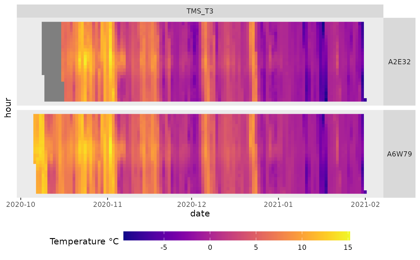
Function plots data with ggplot2 geom_raster. Plot is returned as ggplot faced raster and is primary designed to be saved as .pdf file (recommended) or .png file. Plotting into R environment without saving any file is also possible. See details.
mc_plot_raster(
  data,
  filename = NULL,
  sensors = NULL,
  by_hour = TRUE,
  png_width = 1900,
  png_height = 1900,
  viridis_color_map = NULL,
  start_crop = NULL,
  end_crop = NULL,
  use_utc = TRUE
)
Arguments
- data
myClim object see myClim-package
- filename
output with the extension - supported formats are .pdf and .png (default NULL) If NULL then the plot is shown/returned into R environment as ggplot object, but not saved to file.
- sensors
names of sensor; should have same physical unit see
names(mc_data_sensors)- by_hour
if TRUE, then y axis is plotted as an hour, else original time step (default TRUE)
- png_width
width for png output (default 1900)
- png_height
height for png output (default 1900)
- viridis_color_map
viridis color map option; if NULL, then used value from mc_data_physical
"A" - magma
"B" - inferno
"C" - plasma
"D" - viridis
"E" - cividis
"F" - rocket
"G" - mako
"H" - turbo
- start_crop
POSIXct datetime in UTC for crop data (default NULL)
- end_crop
POSIXct datetime in UTC for crop data (default NULL)
- use_utc
if FALSE, then the time shift from
tz_offsetmetadata is used to correct (shift) the output time-series (default TRUE)In the Agg-format myClim object
use_utc = FALSEis allowed only for steps shorter than one day. In myClim the day nd longer time steps are defined by the midnight, but this represent whole day, week, month, year... shifting daily, weekly, monthly... data (shift midnight) does not make sense in our opinion. But when user need more flexibility, then myClim Raw-format can be used, In Raw-formatuse_utcis not limited, user can shift an data without the restrictions. See myClim-package
Value
list of ggplot2 objects
Details
Saving as the .pdf file is recommended, because the plot is optimized
to be paginate PDF (facet raster plot is distributed to pages), which is especially useful
for bigger data. In case of plotting multiple sensors to PDF, the facet grids are grouped by sensor.
I.e., all localities of sensor_1 followed by all localities of sensor_2 etc.
When plotting only few localities, but multiple sensors,
each sensor has own page. I.e., when plotting data from one locality, and 3 sensors resulting PDF has 3 pages.
In case of plotting PNG, sensors are plotted in separated images (PNG files) by physical.
I.e, when plotting 3 sensors in PNG it will save 3 PNG files named after sensors.
Be careful with bigger data in PNG. Play with png_height and png_width.
When too small height/width, image does not fit and is plotted incorrectly. Plotting into
R environment instead of saving PDF or PNG is possible, but is recommended only for
low number of localities (e.g. up to 10), because
high number of localities plotted in R environment results in very small picture which is hard/impossible to read.
Examples
tmp_dir <- tempdir()
tmp_file <- tempfile(tmpdir = tmp_dir, fileext=".pdf")
mc_plot_raster(mc_data_example_agg, filename=tmp_file, sensors=c("TMS_T3","TM_T"))
#> [[1]]

#>
file.remove(tmp_file)
#> [1] TRUE
#>
file.remove(tmp_file)
#> [1] TRUE